Focal Gradient Loss: Are we looking at focal loss correctly?

Retinanet is a near state-of-the-art object detector that using a simple adaptive weighting scheme, helps bridge some of the gap between one and two stage object detectors by dealing with inherent class imbalance from the large background set constructed by the anchoring process. Specifically they use Focal Loss

The usage of $(1-p{)}^{\gamma }$down weights the categorical cross entropy loss along with how high $p$is. This is parameterized by $\gamma$, where the higher it is, the greater the down weighting is. In their paper they make it clear this choice of adaptive weighting is arbitrary and could be replaced with other schemes.

The question I pose with this, is does this accomplish their goal? (I asked this a while back in a stack exchange question). Given the lack of response in that post, I decided to investigate this myself. I propose another simple adaptive weighting scheme, but I propose applying the approach onto the gradient directly. I do this because most optimizers use a form of gradient descent $\theta \leftarrow \theta -{\mathrm{\nabla }}_{\theta }L$, and so masking the gradient, directly masks how much is learned by each element. I call this set of losses, focal gradient loss

Comparing the objective functions

Its hard to understand it comparitively with the $StopGradient$function, so first lets look at their gradients

Looking at these, we see the focal-loss is a masked version of adaptive weighting plus a residual, $R(p)$. This is the differentiating factor in the two appraoches. We can rewrite the residual as $R(p)=-\gamma \ast F{L}_{\gamma -1}(p)$. It is difficult to say what this does in the optimization perspective, but in terms of sheer magnitude it will always increase the gradient (because the gradient is always negative), moreso if a loss variant is high. This is difficult to describe intuitively but it may be be seen as an additive adaptive bias. This actually increases the spread if you do the math out which may be seen as a benefit but difficult to say for certain, which is why I perform this experiment.

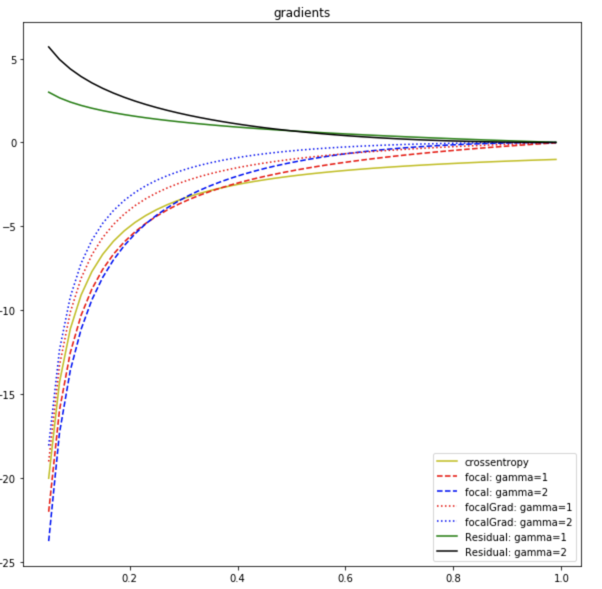
Even though stop_gradient makes it not easily comparable in the loss space, we can integrate its gradient to see its effective equivalent. For values of $\gamma$that arent integers, the integral becomes alot more complicated, so for ease lets just look at the integer case

Note that the bottom bound of the integral is arbitrary, because it only effects the constant, but since we set $FGL(1)=0$from the stop_gradient formulation, I use $z=1$to keep it consistent. Now plotting these we see the following

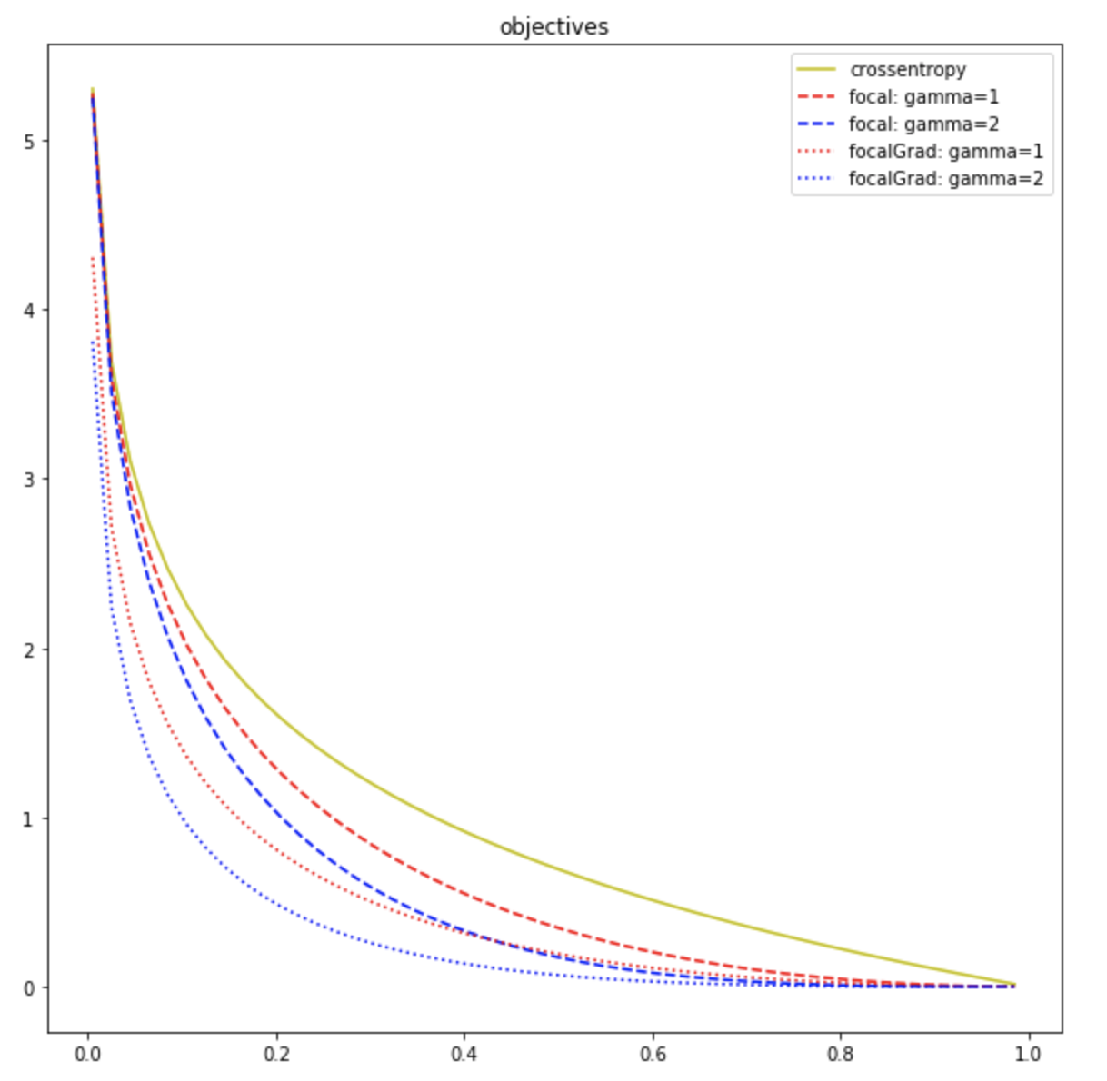
As you can see, focal gradient loss is always lower than the respective focal loss which is understandable based on the spread differential caused by the Residual.

Experiment

Due to computational reasons, we will test on only the setting of $\gamma =2$for 15 epochs on PASCAL VOC 2012. We use the keras-retinanet open source package to do this. Only adjustments I add to the repo is make the custom loss function, and I adjust the training to work with Horovod for more efficient parallelization (I will take any speedups I can get :D)

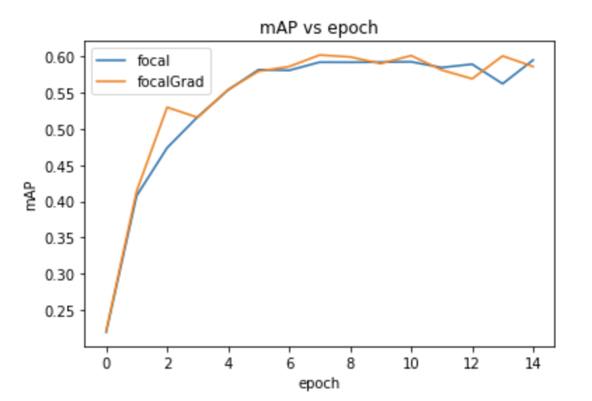
Looking at the results we see they perform similarly. Focal Gradient Loss actually does have a slightly better mAP, but this could be due to noise produced in the training procedure. There is also more noise in general in the Focal Gradient Loss's training compared to Focal Losses-- this may be due to the lack of that additive bias. From this singular (and incomplete) experiment there isnt enough to make conclusions, but if I were forced to do so, I would say the perform similarly but Focal Gradient seems less robust.
I will hopefully be adding more experiments in the future. Stay tuned.