Cubic Step: We Have More Info, Lets Use It!
Hello everyone! In this blog post I introduce an optimizer called Cubic Step where I fit a cubic polynomial to the current and previous step's losses and gradients to solve for the next update. My goal with this post is not to introduce some revolutionary optimizer but rather make aware the lack of the loss function's utility in modern gradient based optimization.
Zeroth order calculations add just as much information about the loss manifold as any other sample, so why is it ignored? This is because most differntiable optimization techniques use gradient based climbing schemes that only care about the local curvature.
Other common techniques like momentum, adagrad, adam, etc. all work on either trying to approximate higher order terms or generate an adaptive learning rate (
Here are some images to examplify the importance of zeroth order info (excuse my terrible drawing):
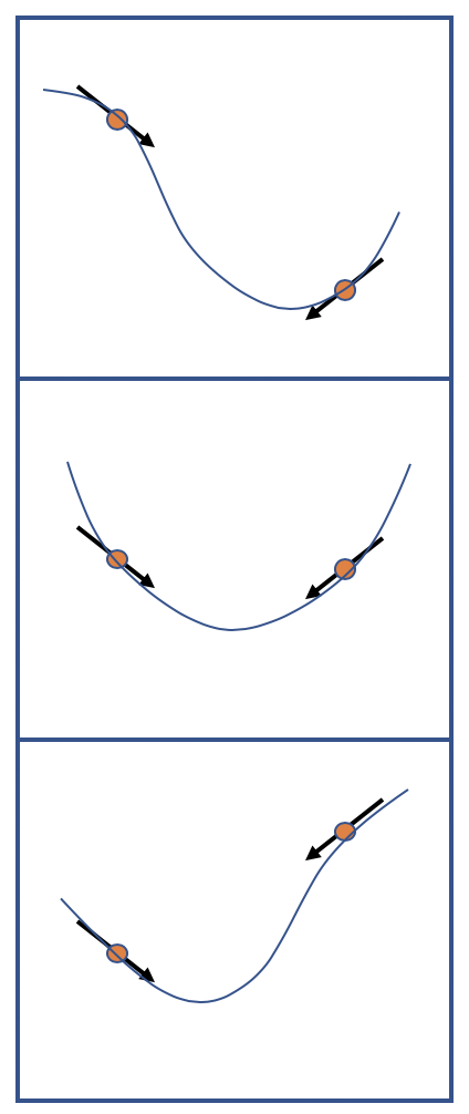
different curves with the same gradients at two samples
Excusing my terrible drawings in the figure, the idea is that even with maintaining first order information, the actual losses change the desired minima. I want to provide a motivating use-case. I devise the Cubic Step optimizer in this post to help deal with oscillations over a critical point in parameter space. The idea is simple, rather than taking a gradient step, I find a cubic that fits the four points
or equivalently:
Its pretty easy to see the inverse exists as long as tf.linalg.inv but that lead to a stream of issues (It worked fine on CPU but on GPU It always caused the program to hang even though I checked that the eigenvalues were numerically stable with respect to floating point precision) so I did what we all had to freshman year of college
Now that we did our little excersize we can actually run the optimizer. Unfortunately this entire scheme makes the difficult assumption that
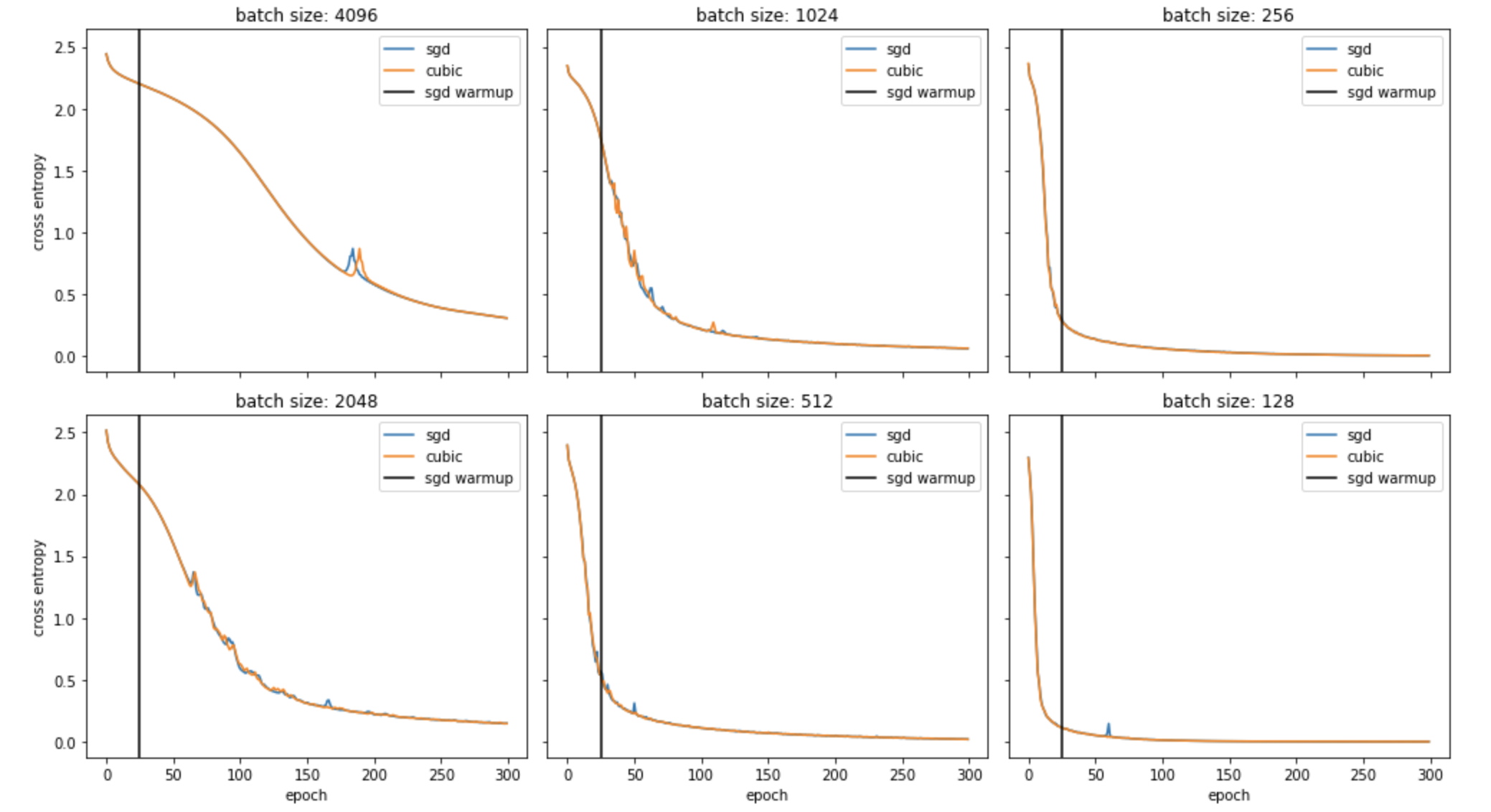
results on a 5 layer CNN on MNIST 4096
These results were interesting and better than I expected. It seems the two methods perfomed nearly the same and for the most part batch percentage had very little effect on the efficacy of Cubic Step and it was also slightly smoother in some cases. The latter was the intended goal, but the former doesnt make much sense given how much this method should be dependant on intra-batch variance. I will atest that probably due to the smoothness of the shallow net's manifold but will require further testing to be sure.
In conclusion the methods worked similarly but I think this result is enough to atleast give all who are reading this enough motivation to atleast keep the idea that zeroth order information is essentially free to access and could be applied in possible future work. Cubic Step only used 4 points, but in reality we can access all previous temporal samples if needed. I chose 4, because cubic was convenient to solve for critical points analytically, while post-5th order is provably impossible as a generality. Actually in a previous post, I go over Focal Gradient Loss as an intuitive competitor of Foal Loss, and that could be seen as an adaptive weighting dependant on zeroth order information too.
I hope you guys enjoyed the post and here is the repo for reproduction and playing yourself with Cubic Step